Startup and a load step
Read current, speed and torque as one connected causal response.
Before you begin: the full motor model and piecewise-constant inputs.
After this lesson you can: analyse derivative changes at a load step and separate startup from a load-response experiment.
Work through the explanation, examples, practical experiment and independent exercises.
Define the experiment
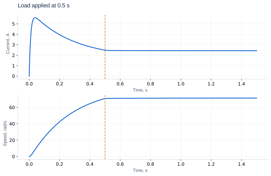
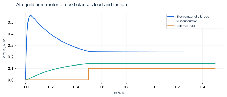
Start the base motor from rest at 12 V, apply ML = 0.1 N·m at 0.5 s and simulate to 1.5 s. Save current, speed, electromagnetic torque and load. Predict the outcome first: load tends to lower speed and raise current. Neither state may jump, but the acceleration changes immediately.
At the start
At t = 0, i = ω = 0. Initial current slope is U/L = 600 A/s; initial acceleration is zero because current has not yet produced torque. Current does not jump to 6 A: that is the stationary-rotor DC value. Back EMF develops during free acceleration and limits the peak. Greater inertia keeps speed low longer and generally makes starting current more demanding.
At the load step
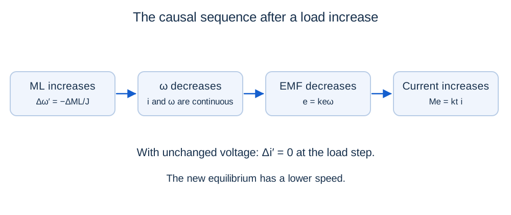
Δi″ = keΔML/(LJ)
For a 0.1 N·m load step, acceleration jumps by −50 rad/s². The one-sided current second derivatives differ by 250 A/s² for the base parameters. This follows from i″ = (−Ri′ − keω′)/L with unchanged voltage. Check these values through the equations rather than noisy numerical differentiation.
Steady droop and measurement
The equilibrium speed change is −14.286 rad/s: 85.714 becomes 71.429 rad/s. Current increases by 0.714 A. At 0.5 s startup has not completely settled, so a load experiment then combines both effects. For a pure disturbance response, initialize at exact equilibrium or wait until a declared settling criterion is met.
Measure starting current over the starting interval and recovery time from the disturbance time. Without a controller, recovery means reaching a new equilibrium, not the old speed. State the reference used for droop and the settling band. If the run ends too soon, report “not settled within the observation interval”; the last sample need not be equilibrium.
Piecewise solution without resetting states
Each constant-input interval has its own equilibrium. If motor parameters are unchanged, A remains the same. Carry the final state into the next interval and measure elapsed time from that interval’s start. This handles voltage steps, pulses and successive load changes.
A reduced-model prediction
Δi(t) ≈ −(ke/R)Δω(t)
One effective time constant after a 0.1 N·m step, speed has fallen about 9.030 rad/s. Final values match the full model, but the initial current dynamics do not: the reduced model changes i′ immediately. Distinguish static droop from maximum dynamic deviation; with oscillations, speed can dip below its new equilibrium.
Independent exercises
1. Remove a 0.1 N·m load from equilibrium at 12 V. Find the new equilibrium and acceleration jump.
Show solution
New speed is 85.714 rad/s and current 1.714 A. Acceleration jumps by +50 rad/s². At the switching instant the old 71.429 rad/s and 2.429 A remain continuous.
2. In the reduced no-load equilibrium model, apply 0.1 N·m for 0.2 s, then remove it. Find speed deviation on removal.
Show solution
Δω = −14.286[1 − exp(−0.2/0.2857)] ≈ −7.192 rad/s. After removal it decays toward zero with the same time constant; do not reset the state.
Practical work
Compare load application at 0.1, 0.5 and 2 s with identical motor parameters. Explain the different initial states. Repeat with changed inertia and load amplitude. Plot Me − ML − bω to verify the approach to mechanical equilibrium.
Calculated illustrations
Key takeaways
Predict physical behaviour before plotting. Separate instantaneous derivative changes from continuous states and distinguish startup from disturbance response.
Progress is stored only in this browser.