Digital control and delays
Exact discretization, digital PI, computation delay, quantization and z-plane stability.
Before you begin: state-space models, PI control and numerical methods.
After this lesson you can: distinguish sampling from integration and evaluate delay and quantization effects.
Work through the explanation, examples, practical experiment and independent exercises.
Three different time scales
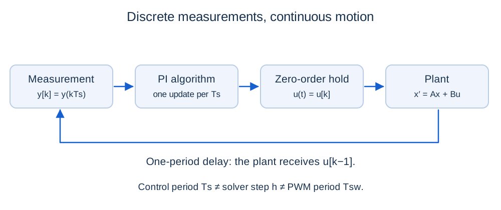
The controller reads sensors every Ts, computes a command and holds it until the next update. PWM has period Tsw, while the model solver has step h. They may coincide numerically but have different meanings. Reducing h does not accelerate a controller with fixed Ts. Update PI only at kTs; integrate the continuous plant between updates with a held command.
An exact zero-order-hold model
Ad = exp(ATs); Bd = ∫₀ᵀˢ exp(Aξ)B dξ
Bd = A⁻¹(Ad − I)B requires invertible A. The exponential of the block matrix [A B; 0 0] also handles integrators. Multiple inputs require multiple B columns, including the load channel. For the RL plant:
i[k+1] = ai[k] + gu[k]
At R = 2 Ω, L = 0.02 H and Ts = 1 ms, a = 0.904837 and g = 0.047581 A/V.
The effect of one sample of delay
No delay: z = a − gK; 0 < K < (1 + a)/g
One-sample delay: z² − az + gK = 0; K < 1/g
Exact discretization preserves plant stability, but digital feedback can destabilize the loop. For positive gain and 0 < a < 1, the base limits are 40.033 V/A without delay and 21.017 V/A with one-sample delay. At K = 30 V/A, the no-delay pole is −0.5226, while delayed complex poles have magnitude 1.1948. Saturation may bound amplitude without making the linear loop stable.
PI update order
u[k] = clip(uraw[k],umin,umax)
v[k+1] = v[k] + Ts{Ki e[k] + [u[k] − uraw[k]]/Tt}
This computes the output before updating the integrator. Reversing those operations defines a different digital controller. Trapezoidal integration uses both current and previous error and needs consistent indexing. Anti-windup also has dynamics: its isolated saturated correction with fixed error requires 0 < Ts/Tt < 2 for explicit-step decay.
Delay, phase and quantization
Encoder speed increment Δω = 2π/(NTs)
At a 200 rad/s crossover, 1 ms delay contributes −11.46°. That is not the complete phase margin: include plant, sensor, controller and hold. Nyquist sampling alone does not ensure good control. An encoder with 2048 actual decoded counts/revolution and a 1 ms speed window gives 3.068 rad/s per count. A longer window improves speed resolution but adds delay.
A uniform ideal 12-bit ADC spanning −5 to +5 A has bin width 10/4096 = 2.441 mA. The difference between endpoint codes may use 4095 under another scaling convention; bin width uses 2¹². Quantization can sustain small limit cycles in a linearly stable loop.
Independent exercises
1. For λ = −20 s⁻¹, find the exact discrete pole at Ts = 0.01 s. Compare exact and Euler at 0.12 s.
Show solution
At 0.01 s, z = exp(−0.2) = 0.81873. At 0.12 s, exact z = exp(−2.4) = 0.09072, but Euler gives −1.4, an unstable approximation to a stable plant.
2. For 4096 counts/revolution and a 5 ms speed window, find the effect of one extra count.
Show solution
Δω = 2π/(4096·0.005) = 0.30680 rad/s. A longer window improves speed estimation resolution but does not change physical position resolution.
Practical work
Implement speed PI with Kp = 0.3, Ki = 1, Tt = 0.05 s and ±12 V limits. Compare Ts = 1, 5 and 20 ms with and without a one-period command delay. Initial states and previous command are zero; reference is 60 rad/s and a 0.1 N·m load appears at 1 s. Report settling, peak current, saturation and speed error. Add sensor quantization, compare continuous PI, and refine h at fixed Ts.
Key takeaways
The controller acts at separate instants while the plant moves continuously. Model holds and delays explicitly and check both pole stability and nonlinear limits.
Progress is stored only in this browser.